Control Bar Features

The control bar at the top provides tools for data management, selection, density contours, export, and import.

1. Projection Selector

Switch between different dimensionality reduction methods:

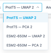
Method	Best For
PCA	Initial overview, finding outliers
UMAP	General exploration, balanced view
t-SNE	Finding clusters
PaCMAP	Fast alternative to t-SNE
MDS	Preserving distances

Different projections reveal different patterns - try switching between them!

URL persistence

Your current projection is reflected in the page URL, so refresh, browser back/forward navigation, and shared links reopen the same view when possible. A bare /explore URL stays unchanged on first load; ProtSpace writes projection and annotation params after you change the view or when it needs to normalize an invalid URL value.

3D Projections

3D projections load normally and are shown as their X/Y view; the third (Z) dimension is not rendered in the web viewer.

2. Annotation Selector

Choose which annotation to use for coloring points:

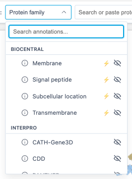
The Annotation dropdown features:

• Grouped categories: Features are organized into sections, one per source (Biocentral, InterPro, TED, Taxonomy, UniProt, Other)
• Search: Type to filter features by name (case-insensitive)
• Keyboard navigation: Use arrow keys to move the highlight, Enter to select, Escape to close. Hovering does not move the arrow-key highlight, and Enter picks the row under the pointer whenever one is hovered.

Only categories present in your dataset appear in the dropdown. Any columns that don't match a known category appear under Other. See the ProtSpace Python package for the complete list of available annotations per source.

⚡ Predicted badge

A ⚡ badge next to an annotation name marks a computational prediction rather than curated or experimental data. Hover it for the tooltip "Predicted: computational, not experimentally curated". The same badge appears next to the legend title when a predicted annotation is active.

Flagged annotations are:

• Signal peptide (Phobius), de-novo topology predictor
• TED domains, domains parsed from predicted AlphaFold structures
• All Biocentral columns: Subcellular location, Membrane, Signal peptide, Transmembrane
• Any other column whose name starts with predicted_

Reference signature-database matches (Pfam, CATH-Gene3D, SUPERFAMILY, SMART, CDD, PANTHER) and curated data (UniProt, Taxonomy) are deliberately not flagged. See Annotations for the full column reference.

STATS badge

A STATS badge marks an annotation that the bundle scored for the projection you are currently viewing. It carries no number; it only says the scores exist. Hover it for the tooltip "Quality statistics available: select this annotation and open the projection metadata panel".

The badge disappears when you switch to a projection the annotation was not scored on. Select the annotation and open the projection metadata panel to read the numbers, or see Separation Scores for what they mean.

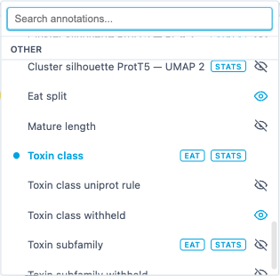
EAT badge

An EAT badge marks an annotation in which some proteins carry a value transferred from a nearby annotated protein instead of a curated record of their own, not to be confused with the ⚡ badge. Hover it for the tooltip "Embedding Annotation Transfer predictions available". Select the annotation to see which proteins those are, and to get the Predicted (transferred) controls in the legend. See Transferred Annotations (EAT) for the whole feature.

Tooltip-only annotations

gene_name, protein_name, and uniprot_kb_id are excluded from the dropdown but are still shown in the tooltip on hover.

3. Search

Find specific proteins by ID:

1. Click inside the search box or press ⌘/Ctrl + K to focus it
2. Type the start of a protein ID (matching is anchored to the start, not anywhere inside)
3. Click a suggestion, or press Enter to take the highlighted row: the first row is highlighted as soon as you type, and the arrow keys move the highlight. Hovering does not move it, so a reflexive Enter on an ID you already selected deselects it
4. An unselected protein joins your selection, the box clears, and the list closes. One that is already selected is listed with a ✓, gains a ✕ on hover or highlight, and is removed instead, leaving your query and the open list in place so you can prune several in a row

Focusing an empty box lists up to 10 proteins from your current selection, mixed in dataset order with the first unselected IDs. An ID the dataset does not contain shows No matching protein IDs found.

Multiple IDs

Paste multiple IDs at once (newline or space separated) and all matching proteins will be selected. Useful for re-selecting a previously exported subset. Pasting a list only ever adds.

4. Selection Tools

Click Select to enter selection mode. A tool picker appears with two options:

• Rectangle (default), drag to draw a box around proteins
• Lasso, draw a freeform outline around proteins

See Box Selection and Lasso Selection for details.

5. Clear Button

Click Clear (or press Escape) to remove all current selections. Pressing Escape again will exit selection mode. Escape while the cursor is in the search box only closes the suggestion list and empties the box; it never clears the selection, however many times you press it.

6. Isolate Button

Isolate focuses on selected proteins by hiding all others:

1. Select one or more proteins (using search, click, or box select)
2. Click Isolate
3. Only selected proteins remain visible
4. Click Reset (appears when isolated) to restore all proteins

Use Case

Isolate is useful for examining relationships within a specific protein subset - hiding unrelated proteins reduces visual clutter.

7. Filter Button

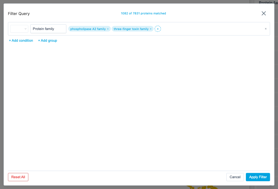
Filter opens a query builder modal for building complex annotation-based filters:

1. Click Filter to open the query builder
2. Each row is a condition: select an annotation, then click + to pick values
3. Combine conditions with AND, OR, or NOT logic
4. Use + Add group for nested logic (parenthetical grouping)
5. The live match count shows how many proteins match your query
6. Click Apply & Isolate to filter the scatterplot

Numeric range conditions

Some annotations hold numbers rather than categories (for example length). When you pick a numeric annotation, the row switches to numeric mode automatically, the + value picker is replaced by a range input. There is no query text to type; you choose an operator and fill in the bound(s):

Operator	Fields shown	Matches
>	min	value strictly greater than min
<	max	value strictly less than max
between	min and max	min ≤ value ≤ max (both ends in)

> is the default operator on a new numeric condition. Switching operators clears any bound the new operator does not use, so a hidden value cannot silently re-constrain the filter.

For example, length between 100 and 300 matches proteins with 100 ≤ length ≤ 300 (both ends included), while length > 500 excludes a protein of exactly length 500.

Comparisons use the raw numeric value, not the legend's bin labels, so the bin settings in the legend do not affect which proteins a numeric condition matches.

A condition with a missing bound matches nothing, and the live match count only appears once the condition is complete.

Missing values

A protein with no value for the annotation never matches >, <, or between. Wrapping the condition in NOT re-includes those proteins, because NOT is the complement of the matched set. There is no numeric equivalent of the categorical N/A entry you can pick from a value list.

Close the modal with the × button, Cancel, Escape key, or clicking the backdrop.

Reset All clears the query and restores all proteins without closing the modal.

Logical Operators

• AND: Protein must match both conditions
• OR: Protein must match either condition
• NOT: Protein must have a value for the annotation and not match the condition

The first condition can optionally be set to NOT for immediate negation.

NOT deliberately excludes proteins with no value (N/A) for the annotation being negated. Negating one protein family, for example, means "belongs to some other family", not "belongs to some other family, or has no family assigned at all". To include unannotated proteins as well, add an explicit N/A condition with OR.

Missing values

Annotations offer presence entries alongside their real values:

• N/A: proteins with no value for this annotation — listed whenever the annotation actually has missing values
• Any value: proteins that have some value — any value at all; always offered

Any value is exclusive: selecting it clears the other values, since "Any value or X" is just "Any value".

Numeric annotations offer the same two entries next to their comparison, so ≥ 0.7 plus N/A reads "at least 0.7, or no score at all". A presence entry on its own is a complete condition — no bounds needed.

Numeric comparisons

Numeric conditions support >, ≥, <, ≤, and between (inclusive on both ends). Missing values never satisfy a comparison — use the N/A entry to include them.

Filter vs Isolate

Both reduce visible proteins, but they work differently:

• Filter: Build annotation-based queries (e.g., "show all Human AND reviewed proteins")
• Isolate: Manually select proteins first, then hide everything else

Use Filter for structured queries. Use Isolate for ad-hoc selections.

8. Export

Click Export to save your visualization:

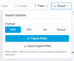
Format	Description
PNG	Raster image with legend
PDF	PDF document with legend
Protein IDs	Text file with newline-separated identifiers
Parquet	.parquetbundle file with all data and optional settings

See Exporting Results for image customization options (dimensions, legend size, font).

9. Import

Click Import to open the menu:

• Load your dataset opens a file picker for a .parquetbundle or FASTA file from your computer. The picker also accepts FASTA files (.fasta, .fa, .fna): ProtSpace sends the sequences to the prep service, which computes embeddings and projections and then opens the resulting bundle automatically. See Importing Data for the full flow, size limits, and privacy implications. You can also drag & drop either file type directly onto the scatterplot.
• Examples lists the startup demo and the datasets behind the ProtSpace paper's figures; Example Datasets describes each one. Each item's label gives the protein count and download size, and its ⓘ icon says what the example is and what its curated view shows, with a link to its section of that page; About these examples above the list links to the whole page. Large examples carry a Large badge, and their ⓘ also gives the download size and the memory and time they take to open. The example currently loaded is disabled, and its ⓘ also appears next to the current dataset's name.

Choosing an example loads it, replaces the dataset stored in your browser (see Data & Settings Persistence), and puts dataset=<id> in the URL, so the link is shareable and the browser's Back button returns to whatever was shown before. The exception is your own import: the menu choice clears it, so Back goes to the entry with no dataset parameter, which loads the demo rather than restoring your import. A link such as /explore?dataset=<id>, with the id from the example's section of Example Datasets, loads the example without touching the stored dataset; visiting the app again without the parameter brings the stored dataset back. An unknown id shows a warning and the app starts up normally.

An example opens on its curated view: the projection, colour-by annotation and tooltip fields chosen for it. A menu choice always opens that view with contours off, so the previous dataset's annotation, projection, tooltip and density parameters don't carry over (Back still returns to them); in a link, those parameters win over the curated ones. As the note under the heading says, changes you make to an example aren't kept: it reopens in its curated state every time.

While an example downloads, the loading screen shows how much of it has arrived and offers Cancel download until decoding starts. Cancelling leaves the current plot and the URL as they were, with no message; on an empty page (a link opened fresh) it removes the dataset parameter and runs the startup load instead. If an example fails to download, whether you chose it from the menu or went Back or Forward to it, ProtSpace shows an error with a Retry button and leaves the current plot and the URL as they were. Only a link opened on an empty page falls back to the startup load.

10. Contours

Contours, the button just right of the search box, draws density rings over the points, so you can see where each category concentrates even where its points pile on top of each other. While Auto or Always is selected, the button is highlighted and names the mode: Contours: Auto or Contours: Always.

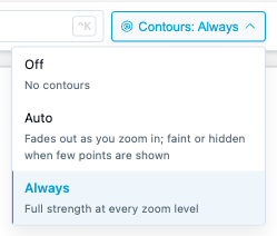
Mode	What it does
Off (default)	No contours
Auto	Fades out as you zoom in; faint or hidden when few points are shown
Always	Full strength at every zoom level

Auto and Always draw the same rings and fill; only their strength differs. Auto sets it from how many points are visible, how large the plot is and how far you have zoomed in. It does not check whether points actually overlap.

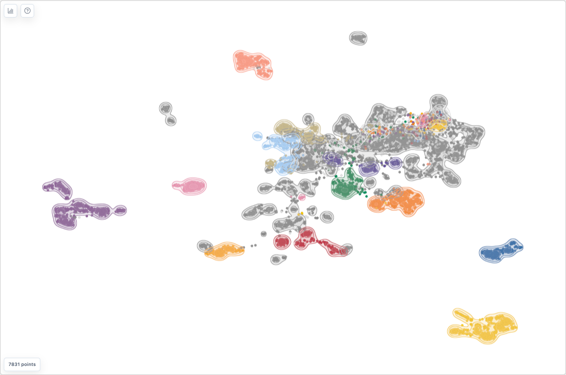
How to read them:

• Every legend colour gets its own set of rings in that colour. Each ring inward marks a doubling of density, and a light fill deepens toward the densest core.
• A spot needs more than 5 points of one colour close together (about 7 piled on one spot) before it gets a ring, so scattered points get none.
• Hidden categories are left out, and selected points are drawn on top of the contours.
• Categories that share a colour share rings. Past 16 colours, the 15 largest keep their own rings and the rest share one grey set. N/A rings are light grey, so they are faint on a light background.
• The rings are computed on a fixed grid across the plot, so they sit in the same place on every screen and at every browser zoom, and lines are equally thick everywhere.

The menu works from the keyboard: with the button focused, Enter or Space opens it, the arrow keys, Home and End move the highlight, Enter picks, and Escape closes it.

Auto on small datasets

Auto counts the visible points. In the full view of a plot about 1000 px wide it shows nothing below about 360 visible points and reaches full strength from about 2,700, and a wider plot needs more. Points you hide, filter out or isolate away do not count. For a small dataset, such as a FASTA upload, or a small subset, pick Always.

URL persistence

The mode is kept in the page URL as density=auto for Auto or density=on for Always; Off leaves the parameter out. A shared link opens with the same mode.

Not in exported images yet

Contours are not drawn in exported images (Quick Export PNG and PDF, the Figure Editor and its zoom insets): the file shows the points only. The Figure Editor preview shows exactly what will be exported. Tracked in #498.

Devices without contour support

Contours need floating-point render targets with float blending (EXT_color_buffer_float and EXT_float_blend), and many iPhone and iPad browsers lack EXT_float_blend. On such a device, or when the graphics driver refuses the contour shaders or buffers, choosing Auto or Always (or opening a link with density=) shows a one-time Contours unavailable notice: "Contours are unavailable on this device, so the Contours setting has no effect. Points are drawn as usual.", followed by the cause in brackets, such as (EXT_float_blend missing). The link keeps its density= parameter, so it still shows contours on a device that supports them.

Tips

• Compare projections: Patterns that appear in multiple projections are more reliable
• Use search: Quickly find known proteins to orient yourself
• Export often: Save interesting views for later

Next Steps

• Viewing 3D Structures - AlphaFold integration
• Exporting Results - Detailed export options