

Using the Legend
The legend panel lets you filter, customize, and explore protein annotations. Most annotations are categorical, but scalar numeric annotations such as length are handled a little differently.
Show And Hide Values
Click any legend row to toggle its visibility:
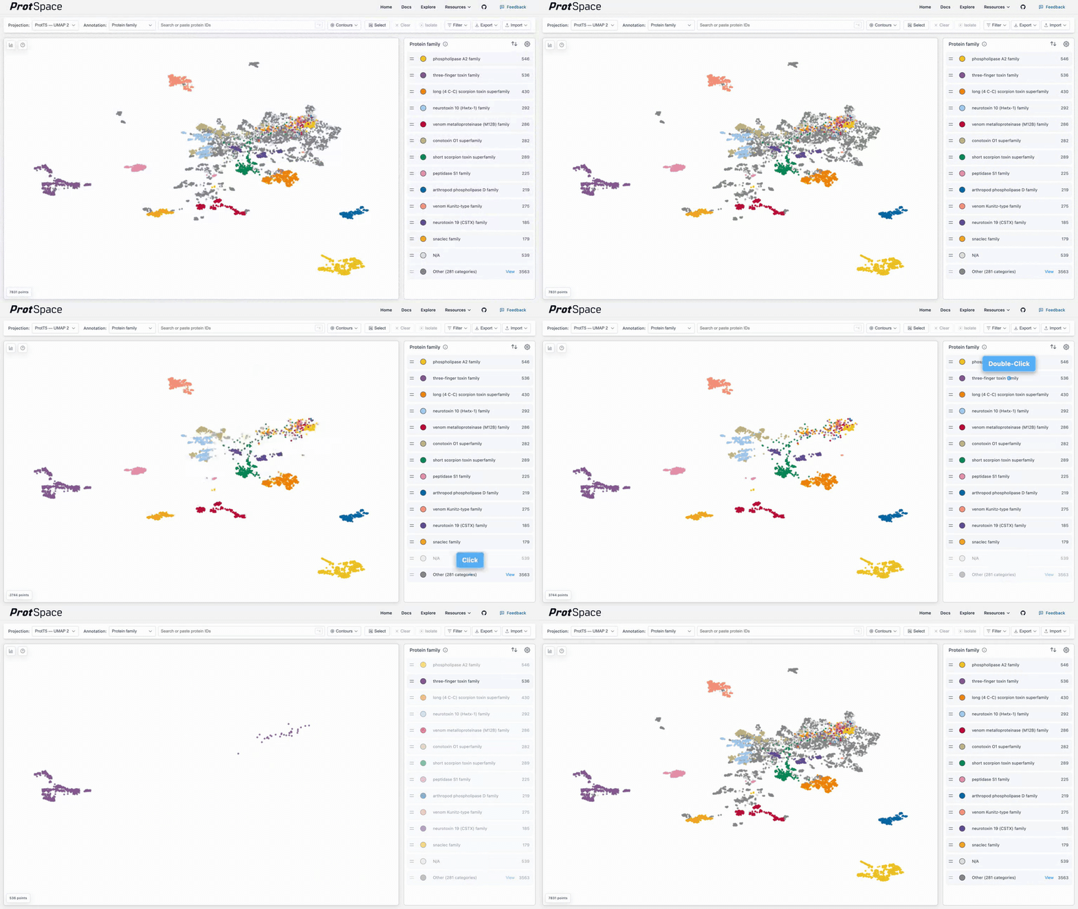
- Click once to hide that value.
- Click again to show it.
- Double-click to isolate that value and hide the rest.
- If only one value remains visible, clicking it restores the full set.
Reordering And Draw Order
Drag labels up or down to change draw order in the scatterplot. Items near the top are drawn on top of items below them.
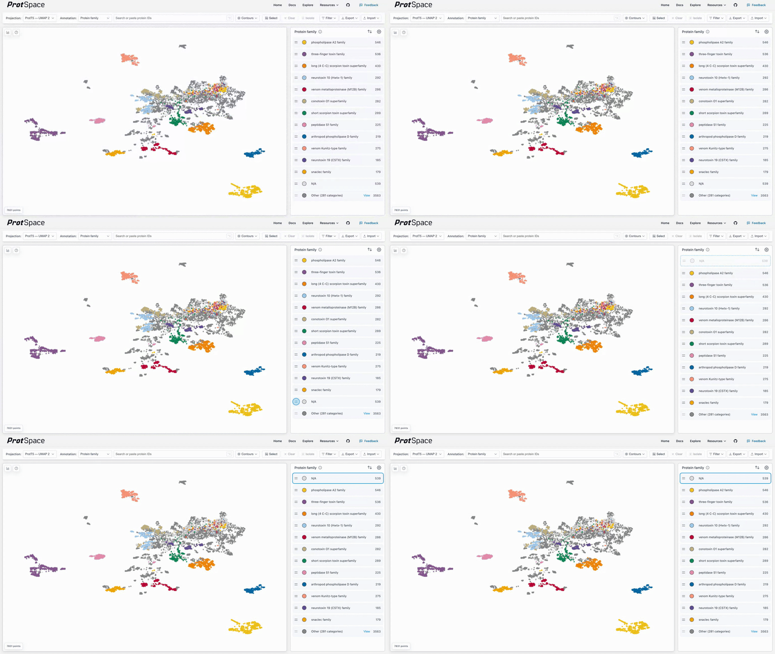
The drag handle stays visible in each legend row so manual ordering is easy to discover. Dragging from any sort mode switches that annotation to Manual order.
The "Other" Group
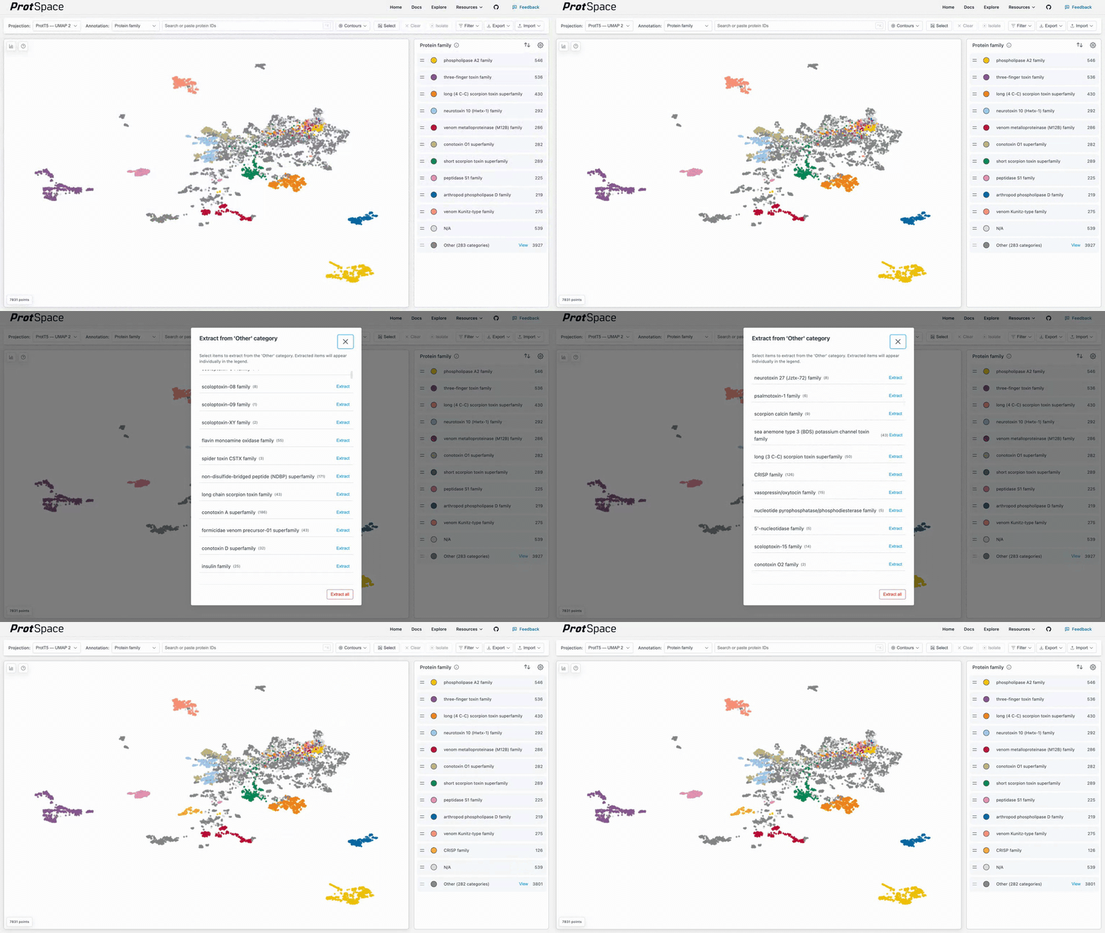
Categorical annotations can group less frequent values into Other once the visible list exceeds the current legend cap.
- Click
Otherto inspect the grouped values. - Extract values from
Otherto show them separately. - Drag values into
Otherto regroup them.
Numeric annotations do not use Other. They are binned directly from the raw numeric values.
Transferred Annotations (EAT)
When the selected annotation carries values borrowed from nearby annotated proteins, a Predicted (transferred) section appears at the very top of the legend panel, above the separation strips. It holds a Show checkbox that adds the borrowed values to the plot and the legend rows, or removes them so those proteins fall back to N/A; a reliability filter — a mode dropdown (Hide below, Hide above, Keep between) with a slider, plus a second slider for the band — that hides predictions falling outside the chosen range; and a count of Observed against Predicted by EAT proteins. Curated values are never hidden by it in any mode, and the section is absent for annotations that have no transferred values.
See Transferred Annotations (EAT) for where the borrowed values come from and how to read them in the plot.
Separation Score Strips
When the dataset was prepared with statistics and the selected annotation was scored in the current projection, two strips appear near the top of the legend panel, above the category list: one for Silhouette, one for Davies–Bouldin. Each plots one dot per category, in that category's legend color, so you can see which values sit apart from the rest and which overlap.
- Hovering a dot highlights the matching legend row, and hovering a row highlights its dot.
- Clicking a dot toggles that category, exactly like clicking its legend row.
- While a filter or isolation narrows the view, the strips are replaced by the note
Separation scores are hidden while the view is filtered.
See Separation Scores for what the numbers mean and how they are computed.
Settings
Click the cog icon in the top-right corner of the legend for advanced options.
Shared Settings
| Setting | What it does |
|---|---|
| Max legend items | Categorical annotations: maximum number of visible values before grouping into Other. Numeric annotations: target maximum number of bins. |
| Shape size / Point size | Adjusts marker size in the scatterplot (range 1 to 64; a larger size from a bundle or an earlier session is capped at 64). The default follows the dataset's protein count, see Default dot size. The size you pick holds for every annotation of the dataset. Numeric annotations use the label Point size because numeric legends always render circles. |
| Show duplicate counts | Shows duplicate count badges and spreads overlapping points when you expand them. |
| Color palette | Picks the active palette for the selected annotation. |
Default dot size
Until you pick a size, the dot size follows how many proteins the dataset has, so a large dataset opens with dots small enough that one category does not cover the others:
| Proteins in the dataset | Up to 10,000 | 20,000 | 40,000 | 100,000 | 570,000 |
|---|---|---|---|---|---|
| Default shape size | 10 | 6 | 4 | 2 | 1 |
The count is the whole dataset, so hiding categories, filtering or isolating does not change it. The settings dialog shows the dataset's default under the size field. To use another size, type it and press Save: it is then stored for the dataset and exported with Include legend settings. A size a bundle sets for an annotation, other than 10 or 30, also overrides the default. To return to the default, clear the size field and press Save. This drops the size you picked and every size a bundle set per annotation, but keeps the annotation's other settings. Reset does the same for the size, and also resets the selected annotation's colors, order and hidden values.
Sorting
Categorical annotations support three sort modes:
By category sizeAlphabeticalManual order
A fourth mode, By separation, appears only when the selected annotation carries per-category separation scores for the current projection, and orders categories by how cleanly each one separates. It is display-only: it reorders the list without changing which categories fall into Other, and it keeps working while the view is filtered.
Numeric annotations support two sort modes:
By numeric valueManual order
The arrow button next to the cog reverses the current sort direction:
- Numeric
By numeric value: low-to-high vs high-to-low - Numeric
Manual order: reverses the current manual order - Categorical
By separation: best-separating first vs worst-separating first - Categorical: preserves the legacy reverse behavior
Numeric Bin Distribution
When the selected annotation is numeric and a numeric gradient palette is active, an extra Bin distribution control appears:
LinearQuantileLogarithmic
Quantile is the default distribution, automatically falling back to Linear when the number of distinct values is small enough that quantile edges would collapse. Logarithmic is only available when all non-null values are strictly positive; otherwise ProtSpace falls back to linear binning.
Reverse Gradient Direction
Numeric annotations also expose a Reverse gradient direction toggle in the settings dialog.
- Off: lower numeric values use the low end of the selected gradient and higher values use the high end.
- On: the gradient is flipped so higher numeric values receive the colors that would normally be used for lower values, and vice versa.
This setting is saved with the rest of the numeric legend settings and is restored on reload or bundle import.
Numeric Annotations
Scalar numeric annotations are stored as raw numbers and binned in the browser from the current numeric settings.
Numeric Labels
Numeric legend labels are display summaries for humans:
- They use
min - maxformatting instead of comparison syntax like<. - Integer-only data stays integer-only in the legend.
- Decimal labels only appear when the source data actually needs decimal precision.
- Single-value bins are shown as a single number.
The exact runtime bin edges are still used for membership. The displayed label is a summary of the values observed in that bin.
Why Fewer Bins Can Appear Than The Max
For numeric annotations, Max legend items is a target cap, not a hard guarantee. You can request 10 bins and still see fewer when the data does not support all of them.
Common reasons:
- A linear or logarithmic interval ends up empty, so it is dropped from the realized legend.
- Quantile cut points collapse because many proteins share the same value.
- A constant numeric column produces exactly one bin.
- An all-null numeric column produces zero bins.
- Very narrow ranges can collapse after precision/topology normalization.
This is why you might see 10 requested bins become 9, and 9 become 8, without anything being wrong.
Predicted Annotations
Some annotations are computational predictions rather than experimentally curated records. When one is selected, the legend header shows a ⚡ Predicted badge next to the annotation title, followed by the note Computationally predicted, not experimentally curated. The same ⚡ marker appears next to the annotation in the control bar's annotation dropdown.
The badge marks columns produced by a machine-learning model, a de-novo sequence-topology predictor, or predicted 3D structure. Reference signature matches such as Pfam, CATH-Gene3D and SUPERFAMILY, and curated or factual UniProt and Taxonomy fields, are not badged. Any unknown column whose name starts with predicted_ is treated as a prediction.
Which built-in columns carry the badge is listed per annotation in the Annotations reference, which is generated from the same table the app reads.
The ⚡ badge is a property of the whole column and is decided from the annotation's name, not from its values, so it is not the same thing as the EAT badge, which marks an otherwise curated column in which some individual proteins carry a transferred value.
Colors, Gradients, And Shapes
Categorical Palettes
Categorical annotations use discrete palettes. ProtSpace keeps the established categorical options for contrast and colorblind safety:
- Kelly's Colors
- Okabe-Ito
- Tol Bright
- Set2
- Dark2
- Tableau 10
Colors stay attached to categories when you reorder them.
Numeric Gradients
Gradients are only shown for numeric annotations. ProtSpace currently ships five curated sequential gradients:
Batlow: scientific-publication oriented sequential ramp from Fabio Crameri's Scientific Colour Maps (default)Cividis: colorblind-friendly sequential gradientViridis: balanced perceptually uniform sequential gradientInferno: high-contrast dark-to-bright rampPlasma: vivid exploratory sequential ramp
These were chosen because they are either perceptually uniform, publication-friendly, accessibility-aware, or visually distinctive for ordered data. Rainbow-style maps are intentionally excluded because they are a poor default for numeric interpretation.
Numeric bin colors are derived from the gradient and the selected distribution. They are not manually edited per bin.
If an imported bundle or saved browser state references an unsupported numeric gradient ID, ProtSpace falls back to batlow.
Special Categories
| Category | Color | Shape |
|---|---|---|
| Other | #999999 | Circle |
| N/A | #DDDDDD | Circle |
Shapes
Every category renders as a circle by default. To assign a different shape (square, diamond, plus, triangle-up, triangle-down) to an individual category, click the category's color/shape swatch in the legend, the popover has a Shape section underneath the color picker.
Numeric and multi-label annotations always render as circles; per-category shape assignment is not available for those.
Saved Settings
Legend settings are saved per dataset and per annotation in the browser.
- Saved examples: visibility, palette, ordering, numeric binning settings, and duplicate-count preferences
- Numeric binning settings such as palette, gradient direction, strategy, and target bin count are restored on reload/import
- Numeric hidden values and manual order are only restored when the current numeric topology still matches the saved one
- The shape size is the exception: it is saved once per dataset, applies to every annotation, and travels in exported bundles with Include legend settings
- Use
Resetin the settings dialog to clear saved preferences for the selected annotation; it also clears the dataset's shape size and every annotation's own size, including sizes a bundle set per annotation, so the default applies to every annotation again
Styling From The Python CLI
protspace style can pre-set legend styling inside a bundle, but its keys are categorical only. For a numeric annotation the web app reinterprets or ignores most of them, because numeric legend entries are bin IDs such as num:quantile:150:200 rather than per-value keys.
Bin distribution and Reverse gradient direction are UI-only settings and cannot be authored from the CLI.
See How CLI keys are reinterpreted for numeric columns for the per-key reference.
Multi-Label Annotations
When proteins have multiple values, such as multiple EC numbers:
- Points display as pie charts
- Each slice represents one value
- All unique values appear in the legend
Next Steps
- Separation Scores - the strips at the top of the legend panel, and how well each category separates
- Control Bar Features - projections, filters, export, and import
- Viewing 3D Structures - AlphaFold integration